
Amazon Web Services Pop-Up loft, West Broadway, Soho, Manhattan.
The AWS AI Day
A few weeks ago I attended the Amazon Web Services AI Day at their co-working loft in Soho, Manhattan. The space was very neat and definitely worth checking out if you’re looking for some place to “Code Happy.” But what exactly was this AI Day about? Well, AI of course! But not just Artificial Intelligence in general. In fact, it turned out to be an immersive advertisement experience around the state-of-the-art technologies AWS makes available for developers to use and embed in their consumer apps.
In an effort to better specify these technologies, it is possible to identify three main areas of concern:
|
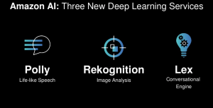 |
Lex
“Amazon Lex is a service for building conversational interfaces into any application using voice and text. Lex provides the advanced deep learning functionalities of automatic speech recognition (ASR) for converting speech to text, and natural language understanding (NLU) to recognize the intent of the text, to enable you to build applications with highly engaging user experiences and lifelike conversational interactions.”

In other words, the Lex API lets developers reinvent the workflows they build, taking advantage of latest technologies for Natural Language Processing, and deploying a User Experience that is closer to how human interactions occur between real people.
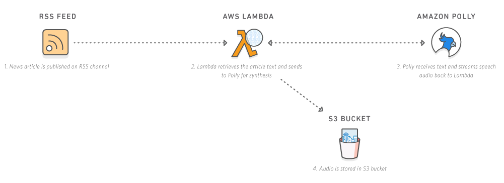
Polly
“Amazon Polly is a service that turns text into lifelike speech. Polly lets you create applications that talk, enabling you to build entirely new categories of speech-enabled products. Polly is an Amazon AI service that uses advanced deep learning technologies to synthesize speech that sounds like a human voice. Polly includes 47 lifelike voices spread across 24 languages, so you can select the ideal voice and build speech-enabled applications that work in many different countries.”
Although Lex and Polly could be seen as the two faces of the same coin, they address two very different problems and have very different responsibilities. While Lex attempts to solve the problem of Natural Language Understanding — a very tough one in AI — Polly aims to “simply” to give a device the ability to “talk” and sound like a human. Not a trivial probem either.
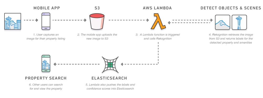
Rekognition
“Amazon Rekognition is a service that makes it easy to add image analysis to your applications. With Rekognition, you can detect objects, scenes, and faces in images. You can also search and compare faces. Rekognition’s API enables you to quickly add sophisticated deep learning-based visual search and image classification to your applications.”
Of the three AWS frameworks, Rekognition is by far the most interesting to me. This framework provides a deep learning-based image recognition framework.
A Little Bit of Background
Ever since I took my final project in college, image recognition has been topic of high interest for me.
A few years ago, I was very attracted to this area of study, so I decided to dive into image recognition and computer vision. At the time, I was an undergraduate student at a school of engineering, and I had absolutely no experience (or previous knowledge) of object detection or machine learning. But for my graduation’s final project, I ended up training an object detector that was able to track tree leaves within a live video stream.
I used a library called OpenCV –an opensource framework for computer vision, ranging form image processing to machine learning and object detection / detector training. I had to manually (!) take hundreds pictures of every possible kind of tree leaves (the good examples), and thousands (luckily this time using a pre-existent training set) of other images of the various things that could resemble a tree leaf (the bad examples). So a lot of fun as you can immagine! 🙂
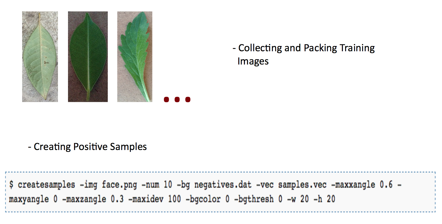
Once you have collected enough good and bad (the majority) examples, you can begin the training of the object detector — which, in my case, is better specified under the name of a Haar-like feature classifier cascade. This algorithm cascades the decisions that the detector must make during the process of image classification — i.e. determine whether an arbitrary object is or is not in the scene of an image — resulting in a positive or negative response.
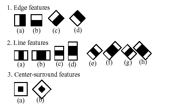
It starts with a “search window,” which spans through the entire area of the image, also scaling its size. At each scan it compares the portion of the image, in the selected window, with a set of key features. Then, stage after stage, it repeats the process with different sets (or variations) of key features (see the image below), and if the comparison results in a positive response, the classifier proceeds (or cascades) to a further stage of analysis. If every stage succeeds, then the object is detected in the image.
So how is this type of machine learning different form what the AWS Rekognition framework uses these days?
Machine Learning and Deep Learning
The first thing we must notice is that, in the field of ML, there are many ways and many approaches that try and address the problem of classifying / detecting / labeling a visible object in an image. Statistical Models, Normal Bayes Classifiers, K-Nearest Neighbors, Support Vector Machines, Decision Trees, Neural Networks, and so on. These are the machine learning algorithms that are provided as part of the OpenCV framework.
In my former project, I had to train a boosted Haar-like features classifier cascade to recognize certain objects (leaves) in an image. Whereas, behind the AWS Rekognition framework there’s the virtually infinite power of Convoluted Neural Networks (CNN) and a huge volume of data (data sets in the order of 10^6 images). One that only years of profile analysis on millions of customers can achieve!
Throughout the entire conference, each and every speaker had seemed to dismiss — as “it’s just magic” — the request for comment on their Deep Learning approach and how they architected their ConvNet (I guess for obvious IP reasons).
However, for the purpose of this article, it makes sense to try demystifying what Deep Learning really means.
Deep Learning Demystified
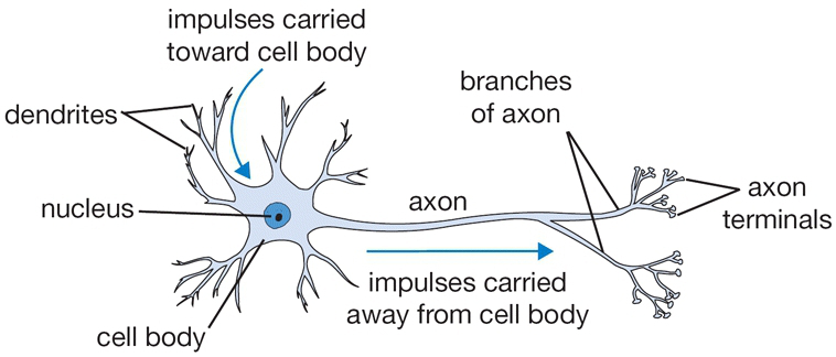
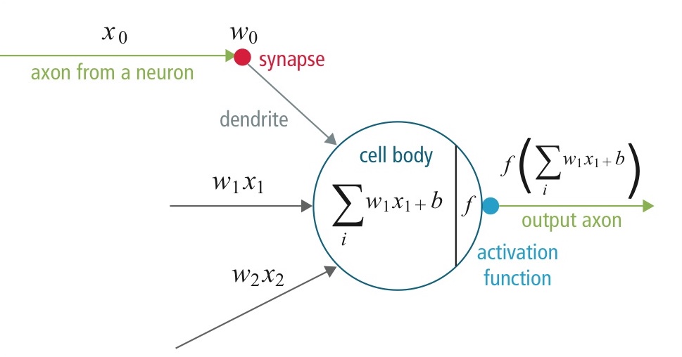
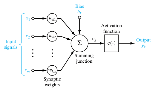
Neural Networks take their name from the resemblance, indeed, they have with the web of neurons in the brain tissue. First, let’s describe the node of a Neutral Network. Just like a neuron, a node has many input channels (dendrites) and one output channel (axon), from which it forwards signals.
Now, we can schematize our neuron (node) into a diagram, simplifying and isolating the inputs from the core and from the output.
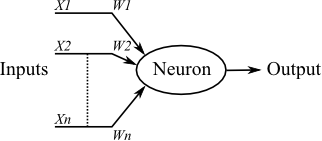
So, after a little bit of thinking, we see that it is just a representation of a function that takes n inputs, combines them, and spits out an output.
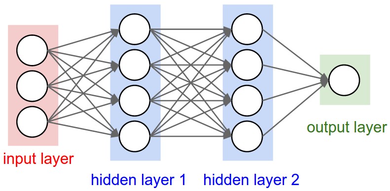
And then finally we can combine these kind of nodes into layers, forming a so-called Neural Network.
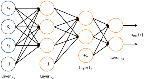
It’s interesting to notice how the nodes in the last picture are aligned in layers. For any given Neural Network, we’ll always have an input layer and an output layer (layers L1 and L4 in the picture). There can also be many layers in between called hidden layers ( L2 and L3 in the picture). The more hidden layers there are, the higher the overall complexity of the Neural Network is, and the Neural Network is thus said to be deep.
CNNs
Very much like regular Neural Networks, Convoluted Neural Networks are made up of neurons that have learnable weights and biases. But CNN architectures make the explicit assumption that the inputs are images, making the forward function more efficient to implement and vastly reducing the amount of parameters in the network.
Neural Networks receive a 1-dimensional input, and transform it through a series of hidden layers, each of which is made up by a set of nodes (neurons) that, in turn, are fully connected with every other node in the previous layer.
Instead, in a CNN, the neurons in a layer are fully connected only to a small region of the previous layer.
Let’s run through a quick example that demonstrates why regular neural networks don’t scale well with images. For instance, if we take a image sized 32×32, the actual input layer’s dimension will be 32x32x3. This is due to the fact that, in the case of an image, we will also have the third dimension associated with the values of the three color channels Red, Green, Blue for each pixel.
Regardless of the “spatial” size (width and height), the input layer associated with an image will always have a depth of 3. So a single neuron in the first hidden layer of a regular Neural Network (a fully-connected neuron) would have 32*32*3 = 3072 weights (or dendrites). For example, an image of size 200x200x3, would have a fully connected layer formed by neurons with 200*200*3 = 120,000 weights each.
The layers of a CNN, instead, will have neurons arranged in 3 dimensions. So every layer of a CNN transforms its 3D input to a 3D output volume of neuron activations. In the image below, the red input layer holds the image, so its width and height are the dimensions of the image, and the depth is 3 (Red, Green, Blue channels).
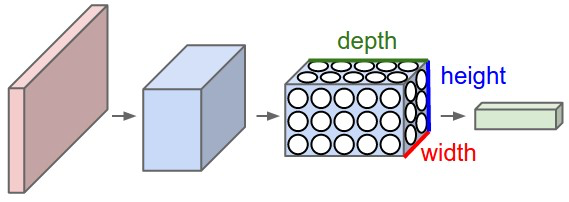
This is an important distinction between regular and convoluted neural networks. But, as we will see soon, is the Convolutional Layer which best characterizes (and indeed names) a Convoluted Neural Network.
By rearranging the layers in this way (in 3D), we have simply redistributed the number of connections (or dendrites) to a neuron, evenly on each of the three values along Z axis of the input volume (along the depth). But there’s more. Instead of connecting each neuron with every other in the input layer, we are now considering only a smaller portion of the input layer (at the time). This is basically convolution. The size of this smaller portion is directly related to the size of the Receptive Field — that is, the size of the filter (or search window [FxFx3]) we had chosen. Notice how the size along the Z axis is constant with the depth of the input volume.
Convolutional Layer
As we started to see, the convolutional layer is made of filters. Each filter is, in other words, a frame — a window which is moved heuristically across the input volume (only varying its position on the X and Y axis, not the depth) and computes a dot product between the input and its relative weight parameter. It’s important to note the distinction between the depth of a filter — that is the depth of the input volume — and the depth of the overall convolutional layer, which is determined by number of filters we choose to use for that layer.
The image below shows an animation of how convolution is executed. Since 3D representations are quite hard to visualize, you can see how each depth slice is arranged across the vertical direction. Meanwhile, from left to right, you see the input volume [7x7x3] in blue, the two filters [3x3x3], and the output volume [3x3x2] in green. As you can guess, the depth of the output volume corresponds to the number of filters in the convolutional layer, where the depth of the filters corresponds to the depth of the input volume.

Click on the image to animate.
In this example, we can synthesize the following:
- the input volume is of size W = [7x7x3]
- the receptive field is of size F = [3x3x3]
- within the size of the input, we have used a zero-padding P = 1
- we apply the filter on the input with a stride S = 2
- the resulting output volume size = [3x3x2] can be obtained as [(W – F + 2P) / S] + 1 = [(7 – 3 + 2) / 2] + 1 = 3
- we have applied a total number of filters (that is, different sets of weights) K = 2
- the depth of the output is indeed equal to the number of the filters used in the convolutional layer
Architecture of a ConvNet
In the process of architecting a CNN, there are many decisions we must make. Among these, are all the hyper-parameters we just described above. In the field of Deep Learning, we are still exploring things in a very early stage, and human knowledge does not yet include a mathematical model which can describe the relations between these hyper-parameters and the resulting performances of a ConvNet. There are, of course, a plethora of best practices and common values for each hyper-parameter. But mainly, researchers do still proceed in an empirical way, in order to find out what combinations of values produce the best results / performances. Some common architectural patterns usually provide small receptive fields (in the order of 3, 5,or 7), a stride of 2, and a zero-pading of 1.
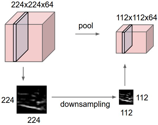
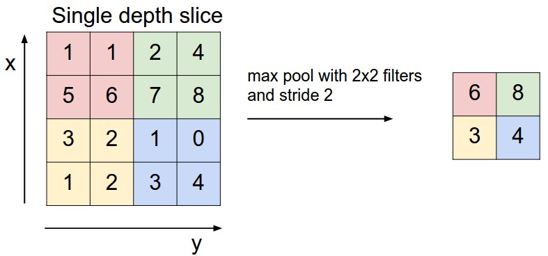
In addition to the Convolutional Layer, it’s worth mentioning the Pooling and ReLU Layer. The first one serves to reduce the amount of complexity. It’s in practice a down-sampling operation for which we usually discard up to the 75% of the information coming out of a Convolutional Layer. There are mainly two types of pooling: Max, and Avg. The first is the used most and works by retaining only the maximum value, out of those other values bounded by the size of the pooling filter.
Even though, historically, the pooling layer has always been adopted (with some caution, otherwise it is too disruptive), we have lately been observing a tendency of discarding such layer, usually in favor of an architecture featuring larger stride values (to reduce the size of the representation), in some Convolutional Layers of the network. It is likely that in the future ConvNets will see fewer to zero use of pooling layers in their implementations.
The other main building block of a ConvNet is — for the sake of completeness — the Rectified Linear Unit (ReLU) Layer. This layer simply performs a max(0, x) element-wise operation, which has the effect of lower-bounding to zero each value of the ReLU’s input volume.
Lastly, I will also mention the Fully-Connected Layer as part (although less often seen) of a CNN’s architecture. This case of layer is quite trivial actually, and it’s simply a regular type of layer in a regular Neural Network, where every neuron is connected to all the neurons of the previous layer.
Most common ConvNet architectures follow the pattern:
INPUT -> [[CONV -> RELU]*N -> POOL?]*M -> [FC -> RELU]*K -> FC
where the * indicates repetition, the POOL? indicates an optional pooling layer, and usually 0 <= N <= 3, M >= 0, 0 <= K <= 2.
In summary:
- In the simplest case, a ConvNet architecture is a list of layers that transform the image input volume into an output volume
- There are a few distinct types of layers (e.g. CONV/FC/RELU/POOL are by far the most popular)
- Each layer accepts a 3D input volume and transforms it to a 3D output volume through a differentiable function
- Each layer may or may not have parameters (e.g. CONV/FC do, RELU/POOL don’t)
- Each layer may or may not have additional hyper-parameters (e.g. CONV/FC/POOL do, RELU doesn’t)
Conclusions and Credits
Although I didn’t want to go too crazy, getting into many implementation details (such as how back-propagation works, for example), I hope that this article serves as appetizer and sparks your curiosity and thirst for knowledge regarding Convoluted Neural Networks and, more generally, the state-of-the-art technologies in Artificial Intelligence and Computer Vision.
So where do we go from here? Well, first of all, I should redirect you to the main sources I used to write this article. The Stanford CS231 class is a great one, it contains a lot of information on this matter (here instead filtered out). I also recommend that you check out this video introduction lecture (special thanks to PhD. Andrej Karpathy), if you don’t exactly feel like investing more time in many of the available readings.